Flatten a Linked List – Brute Force, Merge-Based, and Optimal Approaches

Understanding the Structure and Problem Statement

To tackle this problem, we must first look at the unique node structure. In a standard linked list, each node has a single next pointer. In this problem, every node contains two pointers:

1. next: Connects different sorted linked lists horizontally.
2. child: Connects nodes vertically downwards, forming a sub-linked list.

Crucially, each vertical linked list is already sorted in ascending order. Our goal is to flatten this two-dimensional hierarchy into a single, completely sorted, one-dimensional linked list. By convention, the final flattened list should use the child pointer to link nodes together, while all next pointers are set to nullptr.

Problem Statement

Given a linked list where every node represents a sorted linked list horizontally via the next pointer, and each node has a sorted vertical linked list via the child pointer, flatten the linked list into a single, linearly sorted linked list using only the child pointer.

Example Input

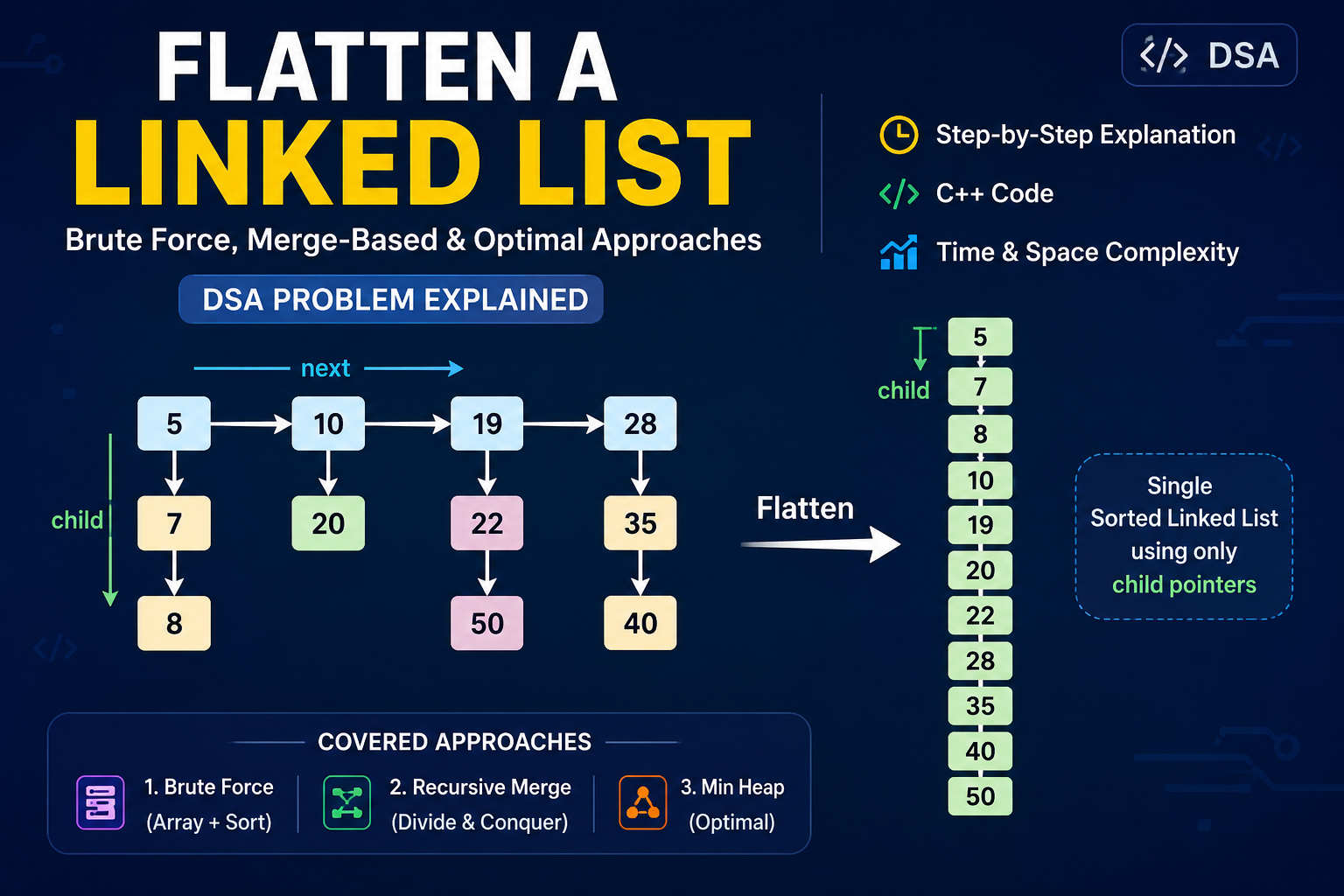
Consider the following structure, where headers are linked via next and vertical columns are linked via child:

5  ->  10 ->  19 ->  28
|       |      |      |
7       20     22     35
|              |      |
8              50     40
|                     |
30                    45

Expected Output

The output should be a single continuous chain linked exclusively by child pointers, sorted completely:

5 -> 7 -> 8 -> 10 -> 19 -> 20 -> 22 -> 28 -> 30 -> 35 -> 40 -> 45 -> 50

The Core Intuition

The foundational challenge here is managing multiple sorted pathways simultaneously. Because each individual vertical column is already sorted, the problem is highly reminiscent of merging multiple sorted arrays or lists.

If we look at the vertical lists as individual streams of sorted data, our task boils down to consolidating these streams into a single sorted river. The structural transition looks like this:

• Input State: A 2D grid of nodes where head points to the top-left item, moving horizontally via next and vertically via child.
• Output State: A 1D sequence of nodes starting from the smallest global element, linked downward via child, with all horizontal next pointers cleared.

Approach 1: Brute Force (Array + Sort)

When confronted with a multi-layered pointer problem during an interview, it is always a safe strategy to start with a straightforward, brute-force approach. It demonstrates your problem-solving mindset and gives you a baseline complexity to optimize against.

Intuition

If the main complication is the two-dimensional nature of the pointers (next and child), we can eliminate that complexity entirely by extracting all the data. We can traverse every single node in the structure, collect their values into a dynamic array (or vector), sort that array using a standard sorting algorithm, and then construct a brand-new linked list from the sorted values.

Algorithm

1. Create an empty dynamic array (e.g., std::vector<int> in C++ or ArrayList<Integer> in Java).
2. Use a nested loop or iterative traversal:
   • Start at the main head node.
   • While the current horizontal node is not null, traverse down its child pointers.
   • Append the value of each node to the array.
   • Move to the next horizontal node via the next pointer and repeat.
3. Sort the array in ascending order using a built-in sorting routine (like std::sort).
4. Create a new dummy head node. Iterate through the sorted array, creating a new node for each value, and link them sequentially using the child pointer.
5. Return the head of the newly created list.

Node* flattenLinkedList(Node* head) {
    if (!head) return nullptr;

    vector<int> arr;

    // Collect all values
    for (Node* h = head; h; h = h->next) {
        for (Node* v = h; v; v = v->child) {
            arr.push_back(v->data);
        }
    }

    sort(arr.begin(), arr.end());

    Node* newHead = new Node(arr[0]);
    Node* cur = newHead;

    for (int i = 1; i < arr.size(); i++) {
        cur->child = new Node(arr[i]);
        cur = cur->child;
    }

    return newHead;
}

Step-by-Step Dry Run

Let's trace this with a scaled-down version of our example:

5 -> 10
|    |
7    12

1. Traversal:
   • Start at 5. Add 5. Move to child 7. Add 7.
   • Move to next header 10. Add 10. Move to child 12. Add 12.
   • nodeValues array becomes: [5, 7, 10, 12].
2. Sorting: The array [5, 7, 10, 12] is already sorted.
3. Rebuilding: A new list is allocated: 5 -> 7 -> 10 -> 12 linked via child.

Complexity Analysis

• Time Complexity: Let $N$ be the total number of nodes across the entire data structure. Traversing all nodes takes $O(N)$ time. Sorting an array of size $N$ takes $O(N \log N)$ time. Rebuilding the list takes $O(N)$ time. Thus, the total time complexity is dominated by the sorting step: $O(N \log N)$.
• Space Complexity: We extract all node values into an array of size $N$, which takes $O(N)$ auxiliary space. Furthermore, constructing a brand-new linked list recreates $N$ nodes, adding another $O(N)$ space overhead. Thus, the total space complexity is $O(N)$.

Advantages & Disadvantages

• Advantages: Extremely simple to understand, trivial to implement, and requires no intricate structural modifications or pointer manipulation.
• Disadvantages: High space complexity. It completely discards the valuable structural trait that individual vertical columns are already sorted. Recreating nodes also wastes memory allocations.

Approach 2: Recursive Merge Approach

To optimize, we must leverage the fact that every vertical list is pre-sorted. This insight allows us to frame the problem as a variation of the Merge Sort algorithm—specifically, the "Merge Two Sorted Lists" subproblem.

Intuition

Instead of trying to handle all columns at the same time, we can break the problem down recursively from right to left.

Imagine we have reached the final two columns on the far right. If we merge those two sorted columns into a single sorted column, we effectively reduce the problem size by one. We can repeat this process moving backward toward the left until the entire grid is consolidated into a single column.

The Role of the Dummy Node

When merging two sorted linked lists, tracking the head of the newly merged list can get messy because the smaller initial value could come from either list. To bypass tedious conditional pointer checks, we use a dummy node.

A dummy node acts as a temporary, fixed structural anchor. We append all sorted nodes directly to the dummy node's child pointer. Once the merge operation completes, the actual head of our merged list lives securely at dummyNode->child. This isolates the merge logic from head-tracking edge cases.

Why Use Only Child Pointers?

The problem requires the output to be a single linear list. Since the columns are structurally organized downward via child pointers, utilizing child pointers to link the final merged list keeps the memory alignment intuitive and satisfies the requirement. The horizontal next pointer of every node in the merged result is explicitly set to nullptr to prevent structural confusion.

Algorithm

1. Base Case: If the head is nullptr or its next pointer is nullptr, return the head (as there is nothing to merge).
2. Recursively move to the end of the horizontal list by calling flatten(head->next). Let the returned head of this flattened remaining list be called flattenedRemainder.
3. Merge the current vertical list (starting at head) with flattenedRemainder using a standard two-pointer sorted merge function.
4. In the merge function:
   • Create a dummy node.
   • Compare nodes from both lists, appending the smaller node to dummy->child.
   • Ensure that for every attached node, the next pointer is explicitly set to nullptr.
5. Return dummy->child as the head of the newly unified column.

C++ Code Implementation

class Solution {
public:
    Node* merge(Node* a, Node* b) {
        Node dummy(-1);
        Node* tail = &dummy;

        while (a && b) {
            if (a->data < b->data) {
                tail->child = a;
                a = a->child;
            } else {
                tail->child = b;
                b = b->child;
            }

            tail = tail->child;
            tail->next = nullptr;
        }

        tail->child = a ? a : b;

        return dummy.child;
    }

    Node* flattenLinkedList(Node* head) {
        if (!head || !head->next)
            return head;

        head->next = flattenLinkedList(head->next);

        return merge(head, head->next);
    }
};

Detailed Dry Run

Let’s walk through a dry run using three short columns:

L1: 5     L2: 10    L3: 19
    |         |         |
    7         20        22

1. flattenRecursive(L1) is called. L1->next is not null, so it calls flattenRecursive(L2).
2. flattenRecursive(L2) is called. L2->next is not null, so it calls flattenRecursive(L3).
3. flattenRecursive(L3) hits the base case because L3->next == nullptr. It returns L3 (the list starting at 19).
4. Execution returns to flattenRecursive(L2). It sets L2->next to the result of L3. Now it calls mergeLists(L2, L3) to combine columns 2 and 3:
   • Compares 10 and 19 $\rightarrow$ 10 chosen.
   • Compares 20 and 19 $\rightarrow$ 19 chosen.
   • Compares 20 and 22 $\rightarrow$ 20 chosen.
   • Remaining 22 attached.
   • Merged result (L2'): 10 -> 19 -> 20 -> 22. This is returned to L1.
5. Execution returns to flattenRecursive(L1). It sets L1->next to L2'. It calls mergeLists(L1, L2'):
   • Combares 5 with 10 $\rightarrow$ 5 chosen.
   • Compares 7 with 10 $\rightarrow$ 7 chosen.
   • The rest of L2' (10 -> 19 -> 20 -> 22) is attached.
6. The fully flattened, sorted list is successfully generated.

Complexity Analysis

• Time Complexity: Let $K$ be the number of horizontal elements (columns) and $N$ be the total number of nodes in the entire grid. Every time we merge two lists, we process their nodes linearly. In the worst-case scenario, we end up merging longer and longer lists repeatedly. The total number of operations scales proportionally to $O(N \cdot K)$. If every column has a length of roughly $M$, then $N = K \cdot M$, making the runtime $O(K^2 \cdot M)$.
• Space Complexity: $O(K)$ auxiliary space. This space is consumed by the implicit recursion call stack, which goes $K$ levels deep down to the last column before unwinding.